A Minimalist PyTorch Physical Adversarial Patch Attack

2021, Dec 10    

Introduction

Visual object classification is a problem of intrinsic interest to humans, other animals, and machines. In line with Moravec’s paradox, this task which seems natural to even relatively simple animal brains proves impossible without specialized and expensive computation. Through the triumph of the deep neural network we can imbue classical computers with the ability to generally understand the appearance of a particular class of object.

The key power of a deep neural network lies in its differentiability (as well as its nonlinearity); through the gradient with respect to a particular weight (or other scalar parameter) for a particular input and desired output, we can know with certainty which direction to change that particular scalar parameter to make the realized output closer to the desired output. It turns out, that for a lot of problems, performing this process repeatedly on one input output pair at a time causes deep neural networks to learn representations which anyone would have to admit seem to share the generality achieved by human intelligence on that particular problem domain.

But the gradient is a double edged sword. In their generosity, neural networks and other differentiable functions tell us how we can deceive them. This power can be leveraged to create generative models which transform noise into outputs resembling some desired class of outputs (e.g. faces). This process is known as generative adversarial training. Training the generator is done by tricking another network called the discriminator, itself trained to determine if an image is real(e.g. a real photo of a face) or a forgery created by the generator. Unlike generative adversarial training, to create adversarial patches, we don’t want to make a realistic-looking image that would fool an image classifier, since that wouldn’t be tricking it at all. Rather, we want to find an patch of pixels from the space of possible patches of pixels which doesn’t look to a human like the object class (i.e. toaster, penguin, etc..) but causes the classifier to predict that class when the patch is introduced into an existing image (ideally, even subject to distortions to the patch and image).

This this blog post discusses a free and open source PyTorch implementation of the adversarial patch attack presented in the paper Brown et. al 2018 (https://arxiv.org/abs/1712.09665) The attack is performed against the default PyTorch pretrained instance of VGG-16, as proposed in the paper Simonyan et. al 2014 (https://arxiv.org/abs/1409.1556)

Implementation

The implementation is provided as free and open source software under MIT license and made available here: https://github.com/balisujohn/adversarial-patch-vgg16

Threat Model

We, the attacker, want to create a circular patch, that can be printed out and when introduced to an image, will fool a pretrained copy of VGG-16. We have access to the pre-trained copy of VGG-16 before hand. We assume that we won’t control the lighting in the room the patch attack is conducted in, the properties of the camera used to collect the images containing the physical patch attack, and that we will not have pixel-perfect control of the scaling and orientation of the patch in the image.

VGG-16

VGG-16 is a 1000-class image classifier trained on ImageNet images; it outputs 1000 numbers, or logits, for each image. Each logit corresponds to a particular class of object, a larger value for a particular logit corresponds to a stronger belief by the network that the input image belongs to the class associated with the logit.

Training Regime (Important!)

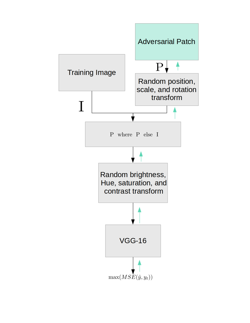
So it’s useful to understand this as a classic supervised learning setup where we use stochastic gradient descent. So just a quick refresher in case it’s helpful; stochastic gradient descent means were here considering one image at a time. For each image we always have the same target action \(y_t\), and the prediction of the network is written as \(\hat{y}\). We will always set all entries of \(y_t\) to -1000 except for the entry corresponding to our target class to 1000. You might think it seems suspicious that we are always encouraging the network to predict the same thing. It seems natural to ask, “might this destroy the existing weights and create a network that always outputs the same thing?” This brings us to the triumph of composed differentiable functions; there is no requirement that we allow all weights to be updated when performing back-propagation. In the above chart, the modules highlighted in green allow parameter updates after the gradients have been calculated, and the grey modules do not. You can clearly see that this training regime cannot modify VGG-16, even though it can use the gradients flowing backward from it (denoted by the green lines). In this way, VGG-16 will serve as our guide in learning how to fool it. So there is only one way that the loss can go down, and that is through the optimization of the parameters in the “Adversarial Patch” module. This module only contains the pixel values of the untransformed patch, represented a square of RGB pixels of fixed size. Maybe you are also suspicious, how does the gradient get all the way back to the “Adversarial Patch” module through the image transformations both before and after the adversarial patch is added to the image. The answer is that every transform used is differentiable, due to the power of PyTorch’s pre-made differentiable image transforms. There is a lot of nondeterminism in these transforms to simulate variations in lighting, patch position, patch distance, and printer color variations.

The Transformation Pipeline, Visualized

Here we show a couple images at each stage in the transformation pipeline, to give a bit more intuition for what is happening as we apply the transforms.

Our starting point

We start with our learnable adversarial patch, and training image

Here is an image of the cute rabbit Momo, which corresponds to \(I\) in the training regime diagram. Note that when actually training, we should have a training-set with many images to sample from.

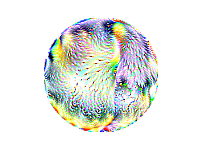
Here is a learnable adversarial patch. This is a RGB square of 200 by 200 pixels, and corresponds to parameters of the green “Adversarial Patch” module in the training regime diagram, as well as its output \(P\). Not that here, this adversarial patch has already been trained a significant amount.

Transforming the Patch

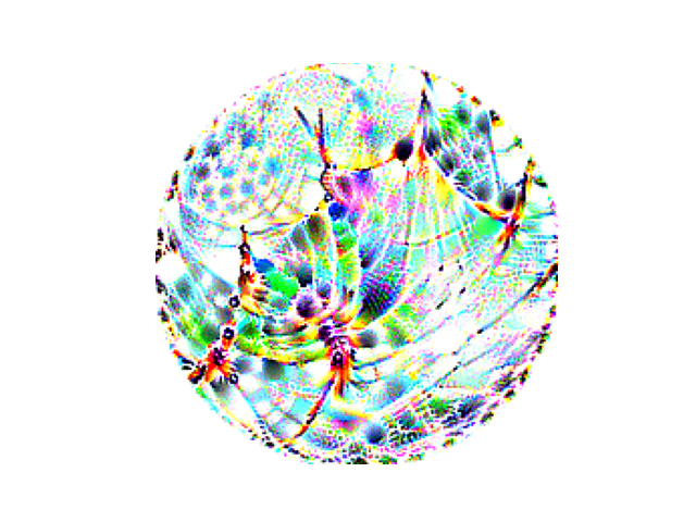
Here are three possible transforms from the distribution of possible transforms applied to the patch before combining it with our training image.

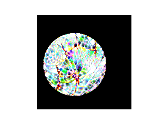
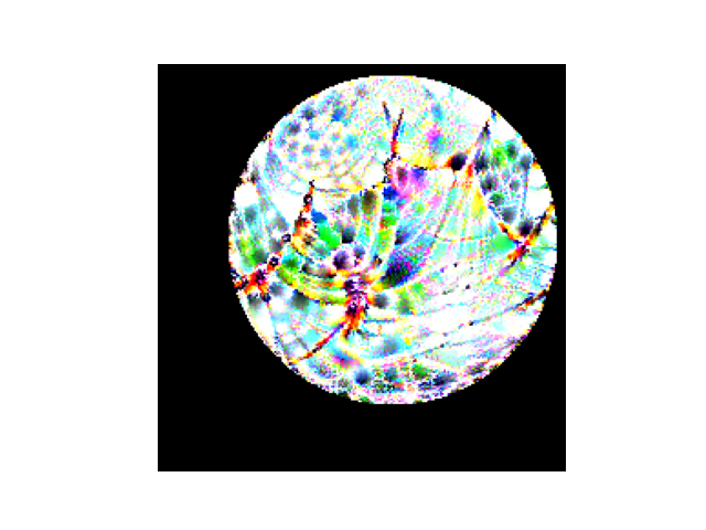
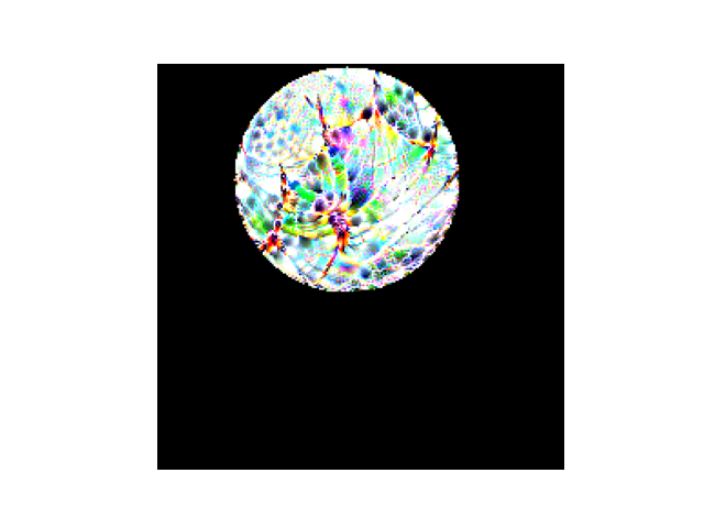
Note that we vary scale, rotation, and position randomly. Note that this is differentiable, so we still have gradients going from the transformed patch to the learnable adversarial patch.

Combination of the Training Image and the Patch

We use the \(P \text{ where } P \text{ else } I\) module to replace the pixels of the training image with the transformed patch where the transformed patch exists (using a binary map since some values of the patch could be zero and we still want to include those)

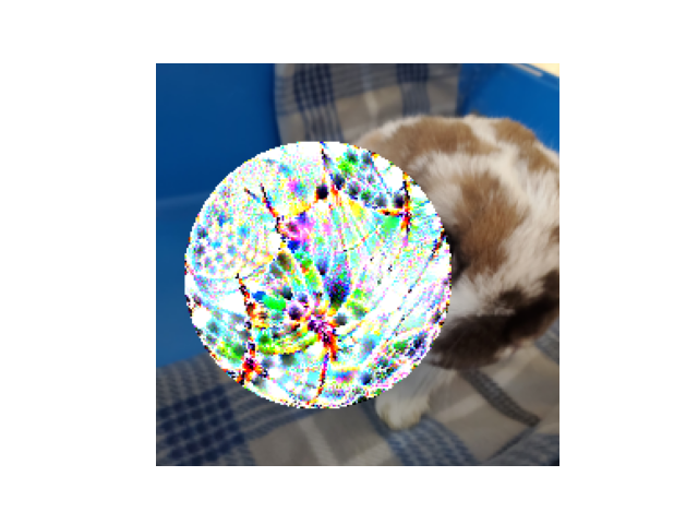
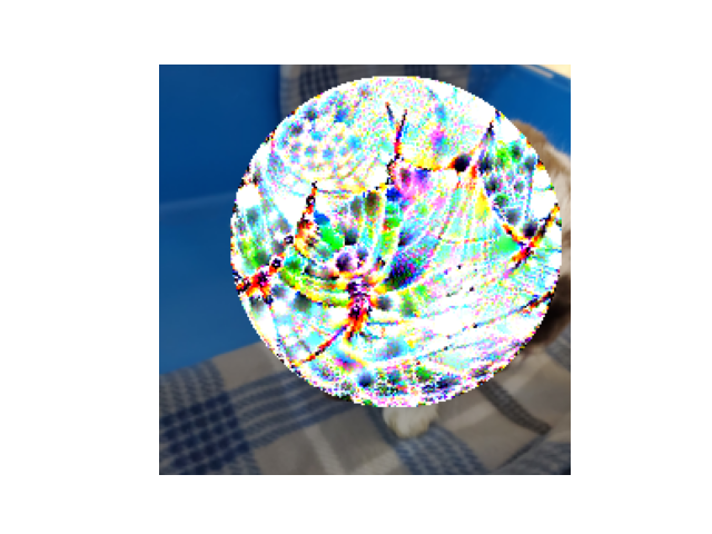
Note that this is also differentiable, so we still have gradients going from the patch-inserted training image all the way back to the learnable adversarial patch.

Image Transforms on the Patch-added Training Image

Finally, we apply random changes to the hue, saturation, brightness, and contrast, in the hope of training a physical patch that will be robust to real-world variations in printers, cameras, and lighting conditions.

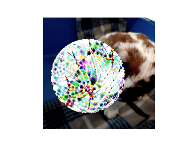
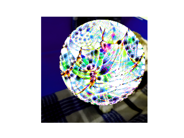
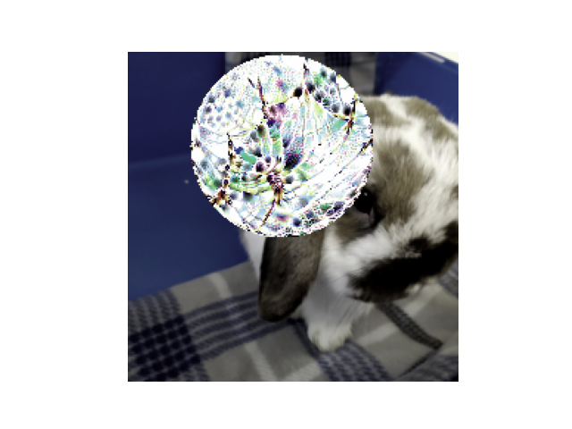
So since we have gradients all the way back from these images, all that remains is to see how VGG-16 classifies these images, then calculate the gradient that reduces (some function measuring distance) between VGG-16’s prediction for each image and the class we want VGG-16 to predict when our patch is introduced to an image. Then we can simply push the pixel values in the adversarial patch in the direction that reduces the loss.

Attack on Live-Webcam VGG-16 classifier

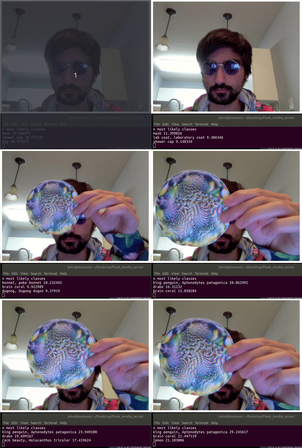
Here is an attack on the default VGG-16 from PyTorch running on a live webcam feed from a Flask server. This patch was trained to cause the classifier to predict the class “king penguin.”

Project Collaborators

John Balis
Harshita Singh

Special Thanks

Special thanks to PyTorch Contributors, Flask Contributors, the authors of Brown 2018 et. al, the authors of Simonyan 2014 et. al, Linux Kernel contributors, Miguel Grinberg for his free and open source webcam Flask server, OpenCV contributors, the creator of this site’s theme, Artem Sheludko, and many other scientists and open source contributors for creating the basis of open science and free and open source software on which this project is built.

Feedback

If you have feedback about this blog-post, feel free to email me at mylastname at wisc dot edu. Alternatively, feel free to directly pull request any corrections to the repository. This whole blog is released under a GPL3.0 license.